Integrate Spectrum (with Baseline Correction)

(adapted from Alan Shusterman, Reed College)

Integrating the spectrum means finding the area underneath the peaks that interest you. This peak area or integral is proportional to the number of hydrogens that create these signals. Therefore, integrals are useful only if we compare them to other integrals. Also, only the relative integral size is meaningful; two integrals with sizes of 1 and 4 tell us the same thing as two integrals with sizes of 0.2 and 0.8.

SpinWorks integration involves four steps. Phasing should have been completed already (but you can rephase peaks at any time). Baseline correction is not usually necessary, and calibration is completely optional. So, if your baseline looks reasonably flat, and your patterns look reasonably well-phased, perform only step 3.

1. Proper phasing (I will assume this has been done already)
2. Correcting baseline for curvature (optional)
3. Selecting integration regions (peaks of interest)
4. Calibrating value of one integral (optional)

2. Baseline correction (optional)

Most spectra contain curved baselines. This curvature look like a broad, low hill stretching across the entire spectrum, or it might look like a sharp, steep twist at one end of the spectrum. In either case, baseline curvature will not usually affect integral measurements much compared to other distorting factors (see above). However, you may occasionally find a spectrum where some compensation for baseline curvature would be helpful, or you just might want to compensate for baseline curvature because that's the kind of careful person you happen to be.

Baseline correction is a procedure that flattens the baseline. First, you tell the program where the baseline is (you do this by clicking on several baseline points). Then, the program looks at the spectrum's height at these "baseline" points, draws a smooth curve that passes through these points, and subtracts this curve from your spectrum. The result is a corrected spectrum in which your selected points lie on the baseline (height = 0), and, you hope, curvature in the original spectrum has been reduced.

• Click on the define baseline points button (this opens a baseline points window containing a Return button)

• Move the cursor to spectrum position that ought to be baseline and click (a short red line will your selection)
  • Repeat this step as desired
• After you have made your selections, click Return in the baseline points window
• Operating tips: If possible, select at least 6 baseline points and space the points across the spectrum so as to produce a useful correction curve (remember that the curve will pass through the selected points). Ideally, select at least one point (and perhaps more) in each "empty" region of your spectrum, and select at least two points in any region that shows a rapidly rising or falling baseline. On the other hand, do not select points close to any NMR signals because the baseline correction will erase some or all of the signal.

• Click Processing: Automatic Baseline (least squares)

3. Selecting integration regions

• Click on the integrate button

At this point, the integration dialog window opens.

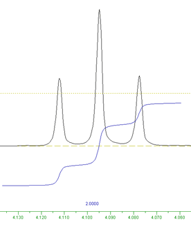
The next step is to define regions for integration. An integration region should consist of: 1) baseline on the left, 2) signals produced by a single type of H in the middle, and 3) baseline on the right. An ideal integration region is shown below. The region extends from the left edge of the blue integral curve to the right edge. If you view integration as a left-to-right procedure, then you can see that the integral curve starts low on the left, remains flat until it approaches an NMR peak, rises as it passes each peak (the degree of curve rise reflects the area under the peak), flattens between peaks, and finishes as a flat line again on the right.

To define an integration region:

• Click on one edge of the region to be integrated (this leaves a red tracking cursor line)
• Click on the other edge of the region to be integrated (a blue integral curve and a numerical value will appear showing the integration region and its area relative to other integrals)
  • Repeat as needed by moving through the spectrum and selecting integration regions
• Operating tip: It can be hard to get integration regions defined properly if you are waving a small cursor arrow over a full spectrum. Adjust the horizontal and vertical scales so that individual peak patterns can be seen in detail, and turn on the tracking cursor (press "t" on the keyboard).
• Operating tip: Do not define overlapping regions.
• Troubleshooting: If you define any integration region incorrectly, click on the integral curve so that a tracking cursor line crosses the integral curve. Click Delete: Current in the integration dialog window.
• After defining all of your integration regions and calibrating one integral curve (see below), click Close in the integration dialog window (the integral curves will vanish, but they will reappear in all printouts!)

• NO REGIONS DEFINED warning: If you clickClose when no integrals are defined, you may cause SpinWorks, and even your computer, to hang, resulting in loss of data. You can avoid this problem by defining at least one region before clicking Close.

4. Calibrate one integral curve (optional)

• Click on the integral curve of interest (this leaves a red tracking cursor line on the curve)
• Set the integral curve's numerical value (usually the #H that you think make these signals) by typing this value in the integration dialog window next to Calibrate
• Click Calibrate in the integration dialog window
• If you have already defined all of the your integration regions, click Close in the integration dialog window (the integral curves will vanish, but they will reappear in all printouts!)

Table of Contents